



Radar Chart HTML CSS JS — SVG Spider Chart
Radar Chart · Charts · Plain HTML, CSS & JS · Live preview
Copy & paste
Source Code
<div class="app">
  <div class="card">
    <div class="card-header">
      <h3>Player Comparison</h3>
      <div class="legend">
        <span class="legend-item"><span class="swatch" style="background:#4a90d9"></span>Player A</span>
        <span class="legend-item"><span class="swatch" style="background:#f5a623"></span>Player B</span>
      </div>
    </div>
    <div class="chart-wrap">
      <svg id="radar" viewBox="0 0 440 400" xmlns="http://www.w3.org/2000/svg"></svg>
    </div>
    <p class="hint">Drag dots to adjust values</p>
  </div>
</div>
* { margin: 0; padding: 0; box-sizing: border-box; }
body { background: #1a1a2e; color: #e0e0e0; font-family: system-ui, sans-serif; min-height: 100vh; display: flex; align-items: center; justify-content: center; }
.app { padding: 20px; }
.card {
background: #16213e; border: 1px solid #0f3460; border-radius: 16px;
padding: 24px; max-width: 500px; width: 100%;
box-shadow: 0 20px 60px rgba(0,0,0,0.4);
}
.card-header { display: flex; justify-content: space-between; align-items: center; margin-bottom: 16px; flex-wrap: wrap; gap: 10px; }
h3 { font-size: 17px; color: #e0e0ff; font-weight: 600; }
.legend { display: flex; gap: 16px; }
.legend-item { display: flex; align-items: center; gap: 6px; font-size: 13px; color: #a0a0c0; }
.swatch { width: 12px; height: 12px; border-radius: 3px; flex-shrink: 0; }
.chart-wrap { overflow: hidden; }
#radar { width: 100%; display: block; }
.hint { text-align: center; font-size: 12px; color: #404060; margin-top: 10px; }const svg = document.getElementById('radar');
const NS = 'http://www.w3.org/2000/svg';
const CX = 220, CY = 200, RADIUS = 150;
const AXES = ['Speed','Power','Defense','Stamina','Agility','Technique'];
const N = AXES.length;
const RINGS = [20,40,60,80,100];
let dataA = [85, 70, 60, 90, 75, 80];
let dataB = [60, 88, 82, 65, 70, 55];
function angle(i) { return (i / N) * 2 * Math.PI - Math.PI/2; }
function pt(val, i) {
const a = angle(i);
const r = (val / 100) * RADIUS;
return { x: CX + r * Math.cos(a), y: CY + r * Math.sin(a) };
}
function tipPt(i) {
const a = angle(i);
return { x: CX + RADIUS * Math.cos(a), y: CY + RADIUS * Math.sin(a) };
}
function el(tag, attrs) {
const e = document.createElementNS(NS, tag);
Object.entries(attrs).forEach(([k,v]) => e.setAttribute(k, v));
return e;
}
function polyPoints(data) {
return data.map((v,i) => { const p = pt(v,i); return `${p.x},${p.y}`; }).join(' ');
}
function hexPts(pct) {
return AXES.map((_,i) => {
const a = angle(i);
const r = (pct/100) * RADIUS;
return `${CX + r*Math.cos(a)},${CY + r*Math.sin(a)}`;
}).join(' ');
}
let dragging = null; // { dataset, idx }
let polyA, polyB, dotsA = [], dotsB = [], labelsA = [], labelsB = [];
function build() {
svg.innerHTML = '';
// Rings
RINGS.forEach(pct => {
const p = el('polygon', {
points: hexPts(pct),
fill: 'none',
stroke: '#1e2d50',
'stroke-width': '1',
});
svg.appendChild(p);
});
// Ring labels (on rightmost axis)
RINGS.forEach(pct => {
const a = angle(1);
const r = (pct/100)*RADIUS;
const t = el('text', {
x: CX + r*Math.cos(a) + 4,
y: CY + r*Math.sin(a) + 4,
fill: '#404060',
'font-size': '10',
'text-anchor': 'start',
});
t.textContent = pct;
svg.appendChild(t);
});
// Axis lines
AXES.forEach((_, i) => {
const tip = tipPt(i);
svg.appendChild(el('line', {
x1: CX, y1: CY, x2: tip.x, y2: tip.y,
stroke: '#1e2d50', 'stroke-width': '1.5',
}));
});
// Axis labels
AXES.forEach((label, i) => {
const a = angle(i);
const r = RADIUS + 22;
const x = CX + r * Math.cos(a);
const y = CY + r * Math.sin(a);
const t = el('text', {
x, y,
fill: '#808090',
'font-size': '12',
'text-anchor': 'middle',
'dominant-baseline': 'middle',
});
t.textContent = label;
svg.appendChild(t);
});
// Dataset A polygon
polyA = el('polygon', {
points: polyPoints(dataA),
fill: 'rgba(74,144,217,0.15)',
stroke: '#4a90d9',
'stroke-width': '2',
'stroke-linejoin': 'round',
});
svg.appendChild(polyA);
// Dataset B polygon
polyB = el('polygon', {
points: polyPoints(dataB),
fill: 'rgba(245,166,35,0.15)',
stroke: '#f5a623',
'stroke-width': '2',
'stroke-linejoin': 'round',
});
svg.appendChild(polyB);
// Animate polygons
[polyA, polyB].forEach(poly => {
const len = poly.getTotalLength ? poly.getTotalLength() : 800;
poly.style.strokeDasharray = len;
poly.style.strokeDashoffset = len;
poly.style.transition = 'stroke-dashoffset 0.8s ease';
requestAnimationFrame(() => { poly.style.strokeDashoffset = '0'; });
});
// Dots A
dotsA = dataA.map((v, i) => {
const p = pt(v, i);
const d = el('circle', {
cx: p.x, cy: p.y, r: '7',
fill: '#4a90d9', stroke: '#fff', 'stroke-width': '1.5',
cursor: 'grab',
});
d.addEventListener('mousedown', e => { e.preventDefault(); dragging = { ds: 'A', idx: i }; });
d.addEventListener('touchstart', e => { e.preventDefault(); dragging = { ds: 'A', idx: i }; }, { passive: false });
svg.appendChild(d);
return d;
});
// Dots B
dotsB = dataB.map((v, i) => {
const p = pt(v, i);
const d = el('circle', {
cx: p.x, cy: p.y, r: '7',
fill: '#f5a623', stroke: '#fff', 'stroke-width': '1.5',
cursor: 'grab',
});
d.addEventListener('mousedown', e => { e.preventDefault(); dragging = { ds: 'B', idx: i }; });
d.addEventListener('touchstart', e => { e.preventDefault(); dragging = { ds: 'B', idx: i }; }, { passive: false });
svg.appendChild(d);
return d;
});
// Value labels A
labelsA = dataA.map((v, i) => {
const p = pt(v, i);
const a = angle(i);
const off = 14;
const t = el('text', {
x: p.x + off*Math.cos(a), y: p.y + off*Math.sin(a),
fill: '#4a90d9', 'font-size': '11', 'text-anchor': 'middle', 'dominant-baseline': 'middle',
});
t.textContent = v;
svg.appendChild(t);
return t;
});
// Value labels B
labelsB = dataB.map((v, i) => {
const p = pt(v, i);
const a = angle(i);
const off = -14;
const t = el('text', {
x: p.x + off*Math.cos(a), y: p.y + off*Math.sin(a),
fill: '#f5a623', 'font-size': '11', 'text-anchor': 'middle', 'dominant-baseline': 'middle',
});
t.textContent = v;
svg.appendChild(t);
return t;
});
}
function updateFromDrag(clientX, clientY) {
if (!dragging) return;
const rect = svg.getBoundingClientRect();
const scaleX = 440 / rect.width;
const scaleY = 400 / rect.height;
const mx = (clientX - rect.left) * scaleX;
const my = (clientY - rect.top) * scaleY;
const dx = mx - CX, dy = my - CY;
const dist = Math.sqrt(dx*dx + dy*dy);
const val = Math.max(5, Math.min(100, Math.round((dist / RADIUS) * 100)));
const { ds, idx } = dragging;
if (ds === 'A') {
dataA[idx] = val;
const p = pt(val, idx);
dotsA[idx].setAttribute('cx', p.x);
dotsA[idx].setAttribute('cy', p.y);
labelsA[idx].setAttribute('x', p.x + 14*Math.cos(angle(idx)));
labelsA[idx].setAttribute('y', p.y + 14*Math.sin(angle(idx)));
labelsA[idx].textContent = val;
polyA.setAttribute('points', polyPoints(dataA));
} else {
dataB[idx] = val;
const p = pt(val, idx);
dotsB[idx].setAttribute('cx', p.x);
dotsB[idx].setAttribute('cy', p.y);
labelsB[idx].setAttribute('x', p.x - 14*Math.cos(angle(idx)));
labelsB[idx].setAttribute('y', p.y - 14*Math.sin(angle(idx)));
labelsB[idx].textContent = val;
polyB.setAttribute('points', polyPoints(dataB));
}
}
window.addEventListener('mousemove', e => updateFromDrag(e.clientX, e.clientY));
window.addEventListener('mouseup', () => { dragging = null; });
window.addEventListener('touchmove', e => {
if (dragging) { e.preventDefault(); updateFromDrag(e.touches[0].clientX, e.touches[0].clientY); }
}, { passive: false });
window.addEventListener('touchend', () => { dragging = null; });
build();Extend with AI
Take This Snippet Further With AI
The AI prompt for this one is for Patreon supporters ($3 a month, 7 days free), along with a site with no ads. Supporters enter the passcode once and it is remembered in this browser.
What's included
Features
About this UI Snippet
How to Build an SVG Radar Chart with Polar-to-Cartesian Math
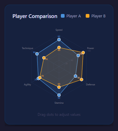
A radar chart — also called a spider or web chart — plots several metrics around a circle, with each axis radiating from the center and the data joined into a polygon. It is the go-to visualization for comparing multi-dimensional profiles like player stats, product scores or skill ratings. This implementation is built with inline SVG and a little trigonometry, supports two overlaid datasets, animates the fill on load, and lets you drag vertices to edit values live. No charting library is used. Here is the full breakdown.
Placing the axes with polar coordinates
The chart has N axes spread evenly around the center, one per metric, separated by 360 / N degrees. The core of the whole chart is the polar-to-Cartesian conversion. For a given axis index i and a radius r (how far out along that axis), the angle is i * (2*PI / N) measured from straight up, and the point is computed as:
x = cx + r * sin(angle) y = cy - r * cos(angle)
Using sin for x and -cos for y (with the minus because SVG's y-axis points down) places the first axis at the top and walks clockwise. A small helper function takes an axis index and a 0-to-1 value and returns the screen point, scaling the value by the chart's maximum radius. Every line, label and data vertex in the chart is positioned through this one function.
The concentric ring grid
The background grid is a set of concentric polygons rather than circles, so the gridlines mirror the data polygon's shape. For each ring level (say 20%, 40%, 60%, 80%, 100%) the code generates a points string by calling the polar helper for every axis at that fixed radius and joining the coordinates with spaces, then renders an SVG <polygon> with a faint stroke and no fill. Straight axis spokes are drawn as <line> elements from the center to each outermost vertex, and axis labels are positioned just beyond the outer ring, with their text-anchor adjusted based on which side of the chart they fall so labels never overlap the shape.
Building the data polygon
Each dataset is an array of values, one per axis, normalized to 0–1. The data polygon's points attribute is built exactly like a grid ring, but using each axis's actual data value as its radius instead of a fixed level. The resulting <polygon> is given a semi-transparent fill and a solid colored stroke. Small <circle> markers are drawn at each vertex so individual values are easy to read and grab.
Overlaying two datasets
Two datasets are rendered as two separate polygons with different colors and translucent fills layered on the same grid, making side-by-side comparison immediate — for example two players' attribute profiles. Because both use the same polar helper and coordinate system, they align perfectly. A legend maps each color to its label.
Animating the fill-in
On load the polygons animate in using SVG stroke techniques. The outline is drawn with a large stroke-dasharray set to the path length and an initial stroke-dashoffset equal to that length, which hides the stroke; transitioning the offset to zero makes the outline appear to draw itself around the shape. The fill opacity is simultaneously transitioned from zero, so the polygon both traces and fades in. This is the standard SVG line-drawing animation applied to a closed polygon.
Draggable vertices for live editing
The chart is interactive: each data vertex marker responds to pointer events. On press, the code records which dataset and axis the grabbed marker belongs to and sets a dragging reference. On move, it converts the pointer position back from Cartesian into a value along that axis — projecting the pointer's offset from center onto the axis direction and dividing by the max radius — clamps it to 0–1, updates the dataset, and rebuilds the polygon and markers. Releasing clears the drag. Because the rebuild reruns the same polar math, dragging a vertex smoothly reshapes the polygon in real time, effectively turning the chart into an input control. Both mouse and touch end events clear the drag state so it works on phones.
Tooltips and labels
Hovering or focusing a vertex can surface the exact value, implemented either through native SVG <title> elements for built-in tooltips or a positioned label. Axis labels and value rings give the chart context without clutter.
Why SVG over canvas here
SVG is ideal for a radar chart because each element — polygon, line, circle, label — is a real DOM node you can style with CSS, animate with transitions, and attach events to individually for dragging and tooltips. The whole chart is just trigonometry feeding coordinate strings into declarative SVG, which makes it crisp at any resolution, accessible, and easy to extend with more axes or datasets by changing the data arrays.
Step by step
How to Use
- 1View the profileSee each metric plotted on its own axis, joined into a polygon over the ring grid.
- 2Compare datasetsRead the two translucent overlays and legend to compare two profiles at a glance.
- 3Watch it animateOn load the polygon outline draws itself and the fill fades in via SVG stroke animation.
- 4Drag a vertexGrab any vertex marker and drag along its axis to change that value live.
- 5Read exact valuesHover or focus a vertex to surface its precise value through a tooltip.
- 6Edit the dataChange the dataset arrays or axis labels in the JS to chart your own metrics.
Real-world uses
Common Use Cases
Got questions?
Frequently Asked Questions
That places the first axis straight up and walks clockwise, which is the conventional radar layout. The minus on cos accounts for SVG y-coordinates increasing downward, so positive values go up the screen.
Concentric polygons share the same vertices as the data shape, so each ring is a scaled copy of the chart outline. This makes it easy to judge a value against the grid and looks cleaner than circular rings behind a polygon.
The pointer position is projected onto the grabbed axis direction and divided by the maximum radius to get a 0-to-1 value, which is clamped and written back to the dataset. The polygon is then rebuilt with the same polar math.
The polygon stroke uses stroke-dasharray equal to its length with an initial dashoffset that hides it. Transitioning the dashoffset to zero makes the outline trace itself, while the fill opacity fades in at the same time.
SVG elements are real DOM nodes, so each vertex can have its own event listeners for dragging and tooltips, be styled with CSS, and animated with transitions. It also stays crisp at any resolution without manual redrawing.
Yes. Use the JSX, Vue, Angular, or Tailwind export buttons on this page. In React, compute the polygon points from your data array with the same polar-coordinate math during render, and pass datasets as props — the SVG re-renders declaratively when values change.