



Scatter Plot — HTML CSS JS SVG Scatter Chart
Scatter Plot · Charts · Plain HTML, CSS & JS · Live preview
Copy & paste
Source Code
<div class="scp-card">
  <div class="scp-head">
    <h3>Study hours vs. exam score</h3>
    <label class="scp-toggle"><input type="checkbox" id="scpTrend" checked> Trend line</label>
  </div>
  <svg class="scp-svg" id="scpSvg" viewBox="0 0 360 240" role="img" aria-label="Scatter plot"></svg>
  <div class="scp-tip" id="scpTip" hidden></div>
</div>*{box-sizing:border-box;margin:0;padding:0}
body{font-family:system-ui,-apple-system,sans-serif;background:#f1f5f9;min-height:100vh;display:flex;align-items:center;justify-content:center;padding:24px}
.scp-card{position:relative;background:#fff;border-radius:16px;padding:22px;width:100%;max-width:460px;box-shadow:0 18px 44px rgba(15,23,42,.08)}
.scp-head{display:flex;align-items:center;justify-content:space-between;margin-bottom:14px}
.scp-head h3{font-size:16px;font-weight:800;color:#0f172a}
.scp-toggle{display:flex;align-items:center;gap:6px;font-size:12px;font-weight:600;color:#475569;cursor:pointer}
.scp-toggle input{accent-color:#6366f1;width:14px;height:14px}
.scp-svg{width:100%;height:auto;display:block}
.scp-grid{stroke:#eef2f7;stroke-width:1}
.scp-axis{stroke:#cbd5e1;stroke-width:1.5}
.scp-pt{fill:#6366f1;opacity:.72;cursor:pointer;transition:opacity .12s,r .12s}
.scp-pt:hover{opacity:1}
.scp-trend{stroke:#ec4899;stroke-width:2;stroke-dasharray:5 4;fill:none}
.scp-tick{font-size:9px;fill:#94a3b8}
.scp-tip{position:absolute;pointer-events:none;background:#0f172a;color:#fff;font-size:12px;font-weight:700;padding:6px 10px;border-radius:8px;transform:translate(-50%,-130%);white-space:nowrap;z-index:5}
.scp-tip[hidden]{display:none}// Each point: [studyHours (0-10), examScore (0-100)]
var DATA = [
[1,42],[2,51],[2.5,49],[3,58],[3.5,62],[4,60],[4.5,71],[5,68],
[5.5,75],[6,79],[6.5,77],[7,85],[7.5,88],[8,86],[8.5,92],[9,95],[9.5,93],
];
var svg = document.getElementById('scpSvg');
var tip = document.getElementById('scpTip');
var card = document.querySelector('.scp-card');
var trendBox = document.getElementById('scpTrend');
var SVGNS = 'http://www.w3.org/2000/svg';
var W = 360, H = 240, PAD = 30;
var XMAX = 10, YMAX = 100;
function sx(x) { return PAD + (x / XMAX) * (W - PAD * 2); }
function sy(y) { return (H - PAD) - (y / YMAX) * (H - PAD * 2); }
function el(n, a) { var e = document.createElementNS(SVGNS, n); for (var k in a) e.setAttribute(k, a[k]); return e; }
// Least-squares linear regression → slope (m) and intercept (b) of best-fit line.
function fit() {
var n = DATA.length, sumX = 0, sumY = 0, sumXY = 0, sumXX = 0;
DATA.forEach(function (p) { sumX += p[0]; sumY += p[1]; sumXY += p[0] * p[1]; sumXX += p[0] * p[0]; });
var m = (n * sumXY - sumX * sumY) / (n * sumXX - sumX * sumX);
var b = (sumY - m * sumX) / n;
return { m: m, b: b };
}
function render() {
svg.innerHTML = '';
for (var i = 0; i <= 5; i++) {
var gy = PAD + i * (H - PAD * 2) / 5;
svg.appendChild(el('line', { class: 'scp-grid', x1: PAD, y1: gy, x2: W - PAD, y2: gy }));
}
svg.appendChild(el('line', { class: 'scp-axis', x1: PAD, y1: H - PAD, x2: W - PAD, y2: H - PAD }));
svg.appendChild(el('line', { class: 'scp-axis', x1: PAD, y1: PAD, x2: PAD, y2: H - PAD }));
// Trend line (best fit) drawn under the points
if (trendBox.checked) {
var f = fit();
svg.appendChild(el('line', { class: 'scp-trend', x1: sx(0), y1: sy(f.b), x2: sx(XMAX), y2: sy(f.m * XMAX + f.b) }));
}
DATA.forEach(function (p) {
var c = el('circle', { class: 'scp-pt', cx: sx(p[0]), cy: sy(p[1]), r: 5 });
c.dataset.x = p[0]; c.dataset.y = p[1];
svg.appendChild(c);
});
}
svg.addEventListener('mousemove', function (e) {
var pt = e.target.closest('.scp-pt');
if (!pt) { tip.hidden = true; return; }
var r = card.getBoundingClientRect();
tip.textContent = pt.dataset.x + 'h → ' + pt.dataset.y + ' pts';
tip.style.left = (e.clientX - r.left) + 'px';
tip.style.top = (e.clientY - r.top) + 'px';
tip.hidden = false;
});
svg.addEventListener('mouseleave', function () { tip.hidden = true; });
trendBox.addEventListener('change', render);
render();Extend with AI
Take This Snippet Further With AI
The AI prompt for this one is for Patreon supporters ($3 a month, 7 days free), along with a site with no ads. Supporters enter the passcode once and it is remembered in this browser.
What's included
Features
About this UI Snippet
Scatter Plot — SVG Point Plot with a Least-Squares Best-Fit Trend Line
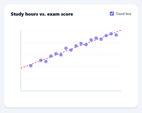
A scatter plot reveals the relationship between two numeric variables — whether they correlate, how tightly, and in which direction. It's the chart you reach for to answer "does X affect Y?" This snippet builds a complete scatter plot in plain HTML, CSS, SVG, and vanilla JavaScript, including an optional least-squares trend line computed from the data itself, gridlines, axes, and hover tooltips — with no charting library.
Plotting points in pixel space
Each data point is an [x, y] pair, and two scaling functions turn data into pixels: sx(x) maps the x value across the padded plot width, and sy(y) maps the y value up the height — inverted, because SVG's y grows downward while the chart's grows upward. Every point becomes a small SVG circle at the scaled coordinates. Because points are real DOM nodes, each one is individually hoverable, which is what lets the tooltip report the exact values behind any dot.
A real best-fit line, not a hand-drawn one
The trend line is computed with least-squares linear regression — the standard method for fitting a straight line to scattered points. fit() accumulates the sums of x, y, x·y, and x² across the dataset, then solves for the slope and intercept with the closed-form formulas. The result is the line that minimises the squared vertical distance to every point: the genuine statistical trend, not an eyeballed approximation. Drawing it from the regression means it updates correctly for any data you feed in.
Toggleable and drawn underneath
A checkbox toggles the trend line on and off, re-rendering the plot. The line is drawn before the points so the dots sit on top of it, keeping them readable and hoverable where the line crosses through the cloud. The line uses a dashed stroke in a contrasting colour so it reads clearly as an overlay rather than as data.
Gridlines, axes, and tooltips
Faint horizontal gridlines and solid x/y axes frame the plot so positions are easy to judge. Hovering any point shows a tooltip with its exact x and y values, positioned at the cursor via getBoundingClientRect, with a single delegated mousemove listener handling every point through closest('.scp-pt'). The tooltip is pointer-events: none so it never steals its own hover.
Data-driven and drop-in
The plot renders from a DATA array of [x, y] pairs, with the axis maxima set by two constants. Swap in your own pairs and the points, scaling, and regression line all follow. Because it's dependency-free SVG, it's crisp at any size, themeable with CSS, and a clear reference for both the data-to-pixel scaling and the linear-regression math that power correlation visualisations.
Step by step
How to Use
- 1Paste HTML, CSS, and JSA scatter plot renders with seventeen points and a best-fit trend line through them.
- 2Toggle the trend lineUse the checkbox to show or hide the least-squares regression line.
- 3Hover a pointMove over any dot to see its exact x and y values in a tooltip.
- 4Swap in your dataReplace the DATA array with your own [x, y] pairs and set XMAX/YMAX to your axis ranges.
- 5Restyle itChange point size, colour, the trend-line dash pattern, or the gridline density.
- 6Wire to an APIFetch your paired values, map them into [x, y] form, and call render() to draw the live chart.
Real-world uses
Common Use Cases
Got questions?
Frequently Asked Questions
It uses least-squares linear regression. fit() accumulates the sums of x, y, x·y, and x² across all points, then applies the closed-form formulas for slope m = (n·Σxy − Σx·Σy) / (n·Σx² − (Σx)²) and intercept b = (Σy − m·Σx) / n. The result is the line that minimises the total squared vertical distance to the points — the genuine statistical best fit, recomputed from whatever data you supply.
Draw order in SVG is paint order — later elements sit on top. Drawing the trend line first means the data points render over it, so where the line passes through the cloud the dots stay visible and hoverable rather than being hidden behind the line. The dashed stroke and contrasting colour further distinguish the line as an overlay rather than data.
Set the XMAX and YMAX constants to the maximum values of your two variables (or a bit above, for headroom). The scaling functions divide by these to map data into the plot area. If your data has a non-zero minimum, subtract the min before scaling and divide by the range (max − min) so the plot uses the full width and height.
As written it assumes a 0-based origin. For negative values, shift the domain: compute min and max, then map (value − min) / (max − min) across the axis, and draw the zero line wherever 0 falls in that range. The point and line drawing stay the same — only the scaling functions change to account for the offset origin.
In React, hold the data and trend-toggle in useState and render circles from .map(), or run render() in a useEffect with a ref; in Vue, use v-for or a template ref with onMounted; in Angular, use *ngFor or ViewChild with ngAfterViewInit. The scaling and regression math is framework-agnostic and ports unchanged — only state and event wiring move into the framework.